What is Microsoft Excel?
Think of Excel like a giant digital notebook made of boxes. Instead of writing on lines, you write inside little boxes called “cells.” Each cell can hold a number, a word, or even a formula (a calculation). Excel then does the heavy lifting — adding, comparing, organizing your data in seconds.
A real-life example: imagine you run a small chai stall. You want to track how much money you made each day. Excel lets you list each day and each amount, and instantly calculates your total earnings for the week — no calculator needed.
When you open Excel, you see a screen with many parts. Let’s explore each one.
The Excel screen — what you’re looking at
Here’s an interactive map of the Excel interface. Click any highlighted area to learn more about it:
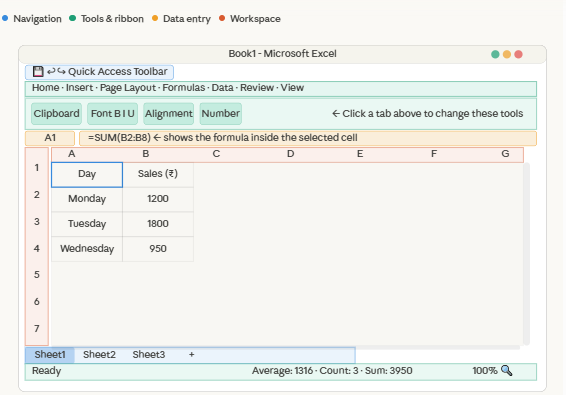
Now let’s go through each part of the interface in detail with simple real-life examples.
Part 1 — The Title Bar
This is the very top of the screen. It shows the name of your file, like “Book1 – Microsoft Excel” or “Chai Stall Sales.xlsx”. When you save your file with a name, this bar updates to show it.
Real example: Just like the cover of your notebook shows its title, the Title Bar shows the name of your Excel file.
Part 2 — The Quick Access Toolbar (QAT)
This is a tiny row of icons at the top-left corner. By default it shows:
- 💾 Save — saves your work
- ↩ Undo — goes back one step (like Ctrl+Z)
- ↪ Redo — brings back what you undid
You can add your own favourite buttons here. For example, if you print a lot, you can pin the Print button here.
Real example: It’s like pinning your most-used apps on your phone’s home screen.
Part 3 — The Ribbon & Ribbon Tabs
The Ribbon is the large toolbar that runs across the top. It is organized into tabs — each tab is a category of tools:
- Home — the most common tools: fonts, colours, alignment, basic number formatting
- Insert — add charts, tables, images, shapes
- Page Layout — control how the sheet looks when printed
- Formulas — find and insert functions like SUM, AVERAGE, VLOOKUP
- Data — sort, filter, and import data
- Review — spell check, comments, protect your sheet
- View — zoom, freeze rows, split windows
Real example: Think of the Ribbon like the control panel of a car. The steering wheel (Home) is right in front; the engine controls (Formulas) are under a different panel. You switch panels depending on what you need.
Part 4 — The Name Box & Formula Bar
These two sit just below the Ribbon and above the spreadsheet.
The Name Box (left, small) shows the address of the currently selected cell. Cell addresses work like coordinates:
- The column letter comes first → A, B, C…
- The row number comes next → 1, 2, 3…
- So “B3” = Column B, Row 3
The Formula Bar (right, long) shows exactly what is inside the selected cell. This is especially important for formulas. If a cell displays “3950” but the formula bar shows =SUM(B2:B4), that means the number was calculated automatically.
Real example: The Name Box is like a GPS telling you “you are here.” The Formula Bar is like lifting the hood of a car — it shows you the engine, not just the speed on the dashboard.
Part 5 — The Worksheet (Cell Grid)
This is the main body of Excel — the grid of boxes. Here is how it’s organized:
Columns run vertically (up and down) and are labeled with letters: A, B, C… up to XFD (that’s 16,384 columns!). Rows run horizontally (left to right) and are numbered: 1, 2, 3… up to 1,048,576 rows. A Cell is where a row and column meet. The cell “B3” is in Column B and Row 3. The Active Cell is the one currently selected — it shows a blue or green border.
Here is a simple example of what a filled worksheet looks like — a chai stall’s weekly sales tracker:
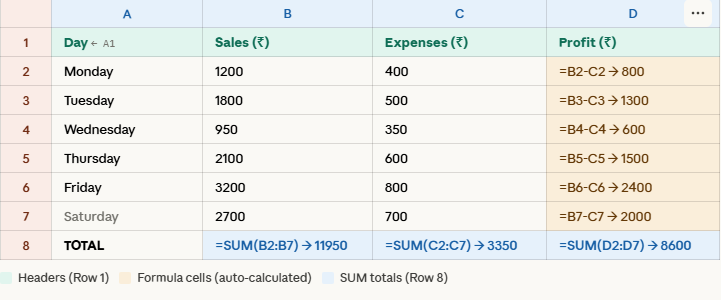
Notice how Column D calculates profit automatically using =B2-C2. And Row 8 sums up everything using =SUM(B2:B7). You type the formula once — Excel does the math every time the data changes.
Part 6 — The Sheet Tabs
At the bottom of the screen, you’ll see tabs labeled Sheet1, Sheet2, Sheet3. One Excel file (called a Workbook) can contain many sheets (called Worksheets).
Real example: Think of an Excel workbook like a multi-subject notebook. Each sheet is one subject’s chapter. A small business owner might use Sheet1 for January data, Sheet2 for February, and Sheet3 for a yearly summary.
You can rename a sheet by double-clicking its tab. You can add a new sheet by clicking the + button next to the last tab.
Part 7 — The Status Bar
The thin bar at the very bottom of the screen is quietly one of the most useful parts of Excel. When you select a group of cells containing numbers, it instantly shows: their Sum (total), their Average, and their Count (how many cells are selected) — without you typing a single formula.
Real example: Select Monday to Saturday’s sales and the status bar immediately says Sum: 11,950. It’s a quick-calculation cheat sheet.
Key Terms to Remember
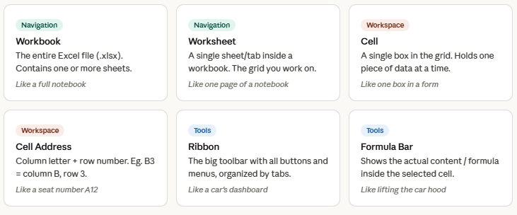
Here is a quick-reference card for the most important vocabulary from this chapter:
Practice Exercise for Students
Try this when you open Excel for the first time:
- Open Excel and look at each part of the screen — can you identify the Ribbon, Name Box, and Formula Bar?
- Click on cell B3. Look at the Name Box — it should say “B3”.
- Type your name in cell A1 and press Enter.
- Click on A1 again — notice your name appears in both the cell and the Formula Bar.
Type the numbers 100, 200, 300 in cells B1, B2, B3. Then click on B4 and type =B1+B2+B3 — press Enter and see the magic!